How Many Different Samples Of Size 4 Can Be Selected From A Population Of Size 8?

The Central Limit Theorem

In Notation 6.5 "Instance 1" in Section six.ane "The Mean and Standard Deviation of the Sample Mean" nosotros synthetic the probability distribution of the sample hateful for samples of size two drawn from the population of 4 rowers. The probability distribution is:

$$\begin{array}{cccccccc}\stackrel{-}{\mathit{x}}& 152& 154& 156& 158& 160& 162& 164\\ P\left(\stackrel{-}{\mathit{ten}}\right)& \frac{\mathrm{ane}}{16}& \frac{2}{16}& \frac{\mathrm{three}}{16}& \frac{4}{16}& \frac{3}{16}& \frac{\mathrm{ii}}{\mathrm{xvi}}& \frac{1}{16}\end{array}$$

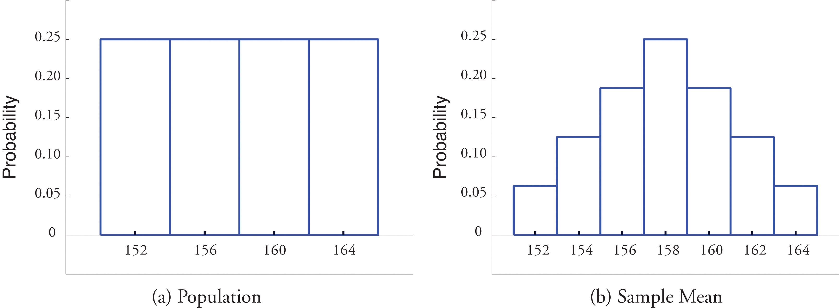
Figure half dozen.1 "Distribution of a Population and a Sample Hateful" shows a side-by-side comparison of a histogram for the original population and a histogram for this distribution. Whereas the distribution of the population is uniform, the sampling distribution of the mean has a shape approaching the shape of the familiar bell curve. This phenomenon of the sampling distribution of the mean taking on a bell shape even though the population distribution is not bell-shaped happens in general. Here is a somewhat more realistic example.

Figure 6.1 Distribution of a Population and a Sample Mean

Suppose we accept samples of size 1, 5, ten, or 20 from a population that consists entirely of the numbers 0 and 1, half the population 0, half one, so that the population mean is 0.5. The sampling distributions are:

n = 1:

$$\begin{array}{ccc}\stackrel{-}{\mathit{x}}\hfill & 0& 1\\ P\left(\stackrel{-}{\mathit{10}}\right)\hfill & \mathrm{0.v}& \mathrm{0.five}\end{array}$$

n = 5:

$$\begin{array}{ccccccc}\stackrel{-}{\mathit{ten}}\hfill & 0& 0.2& 0.4& 0.6& 0.8& \mathrm{ane}\\ P\left(\stackrel{-}{\mathit{x}}\right)\hfill & 0.03& 0.16& 0.31& 0.31& \mathrm{0.xvi}& 0.03\end{array}$$

northward = 10:

$$\begin{array}{cccccccccccc}\stackrel{-}{\mathit{x}}\hfill & 0& 0.1& \mathrm{0.ii}& 0.3& \mathrm{0.iv}& \mathrm{0.five}& 0.6& \mathrm{0.seven}& 0.8& 0.9& 1\\ P\left(\stackrel{-}{\mathit{x}}\right)\hfill & 0.00& 0.01& 0.04& 0.12& 0.21& 0.25& 0.21& 0.12& 0.04& 0.01& 0.00\end{array}$$

n = xx:

$$\begin{array}{cccccccccccc}\stackrel{-}{\mathit{x}}\hfill & 0& 0.05& 0.10& 0.15& \mathrm{0.twenty}& 0.25& 0.30& 0.35& 0.40& 0.45& \mathrm{0.l}\\ P\left(\stackrel{-}{\mathit{ten}}\right)\hfill & 0.00& 0.00& 0.00& 0.00& 0.00& 0.01& 0.04& 0.07& 0.12& 0.16& \mathrm{0.eighteen}\end{array}$$ $$\begin{array}{ccccccccccc}\stackrel{-}{\mathit{10}}\hfill & 0.55& \mathrm{0.sixty}& 0.65& 0.70& 0.75& \mathrm{0.eighty}& 0.85& 0.90& 0.95& \mathrm{ane}\\ P\left(\stackrel{-}{\mathit{x}}\right)\hfill & \mathrm{0.xvi}& 0.12& 0.07& 0.04& 0.01& 0.00& 0.00& 0.00& 0.00& 0.00\end{array}$$

Histograms illustrating these distributions are shown in Figure 6.2 "Distributions of the Sample Mean".

Effigy 6.2 Distributions of the Sample Mean

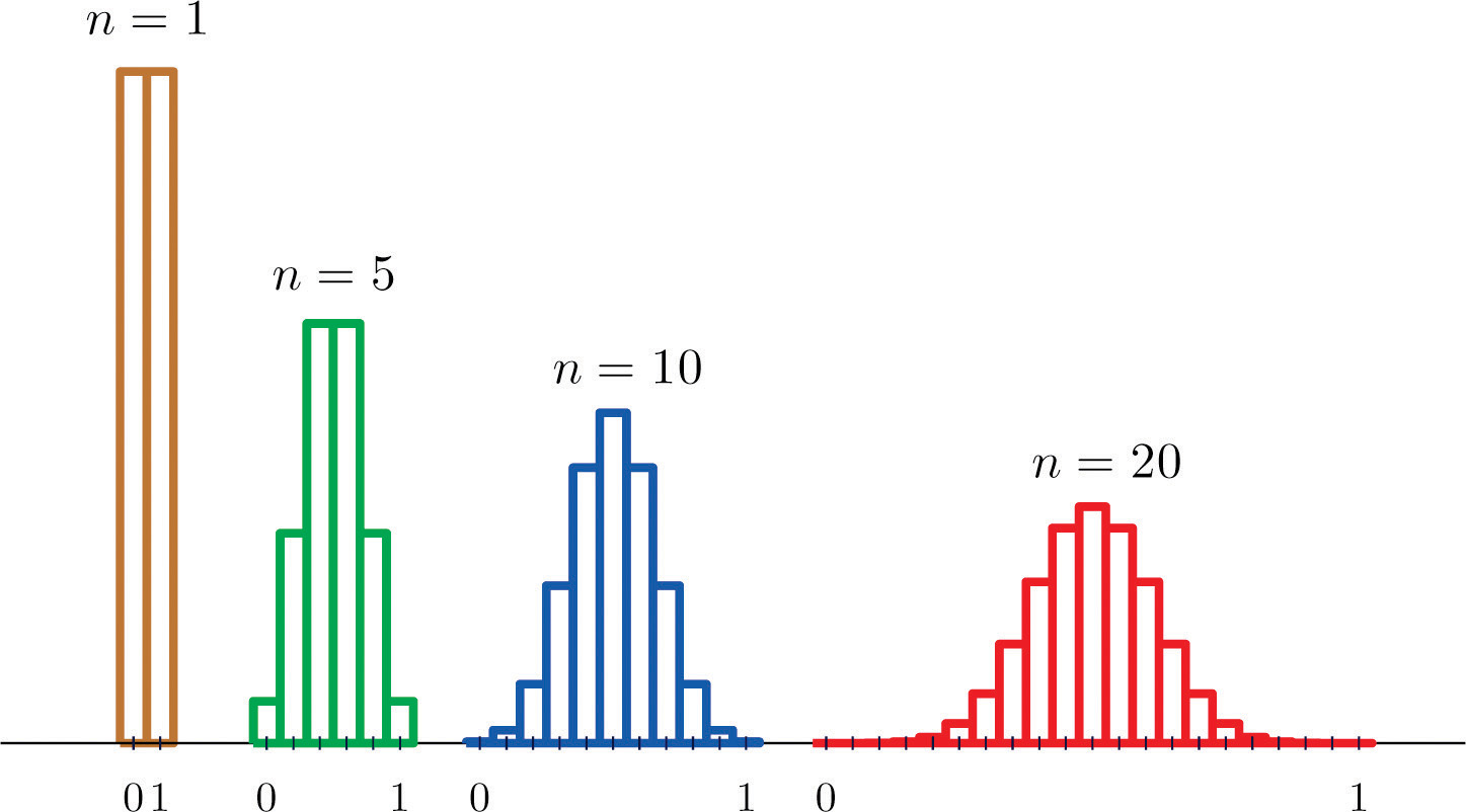
As n increases the sampling distribution of $\stackrel{-}{\mathit{Ten}}$ evolves in an interesting way: the probabilities on the lower and the upper ends shrink and the probabilities in the middle become larger in relation to them. If we were to continue to increase n so the shape of the sampling distribution would go smoother and more than bell-shaped.

What we are seeing in these examples does non depend on the item population distributions involved. In general, one may start with any distribution and the sampling distribution of the sample mean will increasingly resemble the bong-shaped normal bend equally the sample size increases. This is the content of the Cardinal Limit Theorem.

The Central Limit Theorem

For samples of size 30 or more, the sample mean is approximately normally distributed, with mean ${\mathit{\mu }}_{\stackrel{-}{\mathit{Ten}}}=\mathit{\mu }$ and standard deviation ${\mathit{\sigma }}_{\stackrel{-}{\mathit{X}}}=\mathit{\sigma }/\sqrt{n}$ , where northward is the sample size. The larger the sample size, the amend the approximation.

The Central Limit Theorem is illustrated for several mutual population distributions in Figure half dozen.3 "Distribution of Populations and Sample Means".

Figure vi.3 Distribution of Populations and Sample Means

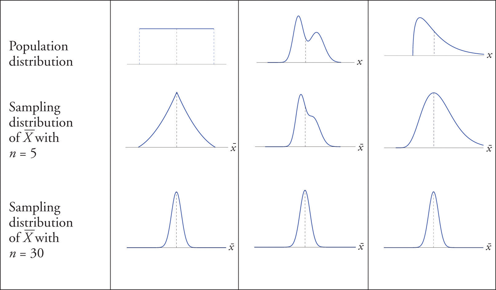
The dashed vertical lines in the figures locate the population mean. Regardless of the distribution of the population, as the sample size is increased the shape of the sampling distribution of the sample mean becomes increasingly bell-shaped, centered on the population mean. Typically by the time the sample size is 30 the distribution of the sample mean is practically the aforementioned every bit a normal distribution.

The importance of the Central Limit Theorem is that it allows us to make probability statements about the sample mean, specifically in relation to its value in comparison to the population mean, equally nosotros will see in the examples. But to use the event properly we must outset realize that there are two divide random variables (and therefore two probability distributions) at play:

1. X, the measurement of a single element selected at random from the population; the distribution of X is the distribution of the population, with hateful the population mean μ and standard deviation the population standard deviation σ;
2. $\stackrel{-}{\mathit{Ten}}$ , the mean of the measurements in a sample of size n; the distribution of $\stackrel{-}{\mathit{X}}$ is its sampling distribution, with mean ${\mathit{\mu }}_{\stackrel{-}{\mathit{X}}}=\mathit{\mu }$ and standard deviation ${\mathit{\sigma }}_{\stackrel{-}{\mathit{Ten}}}=\mathit{\sigma }/\sqrt{\mathrm{north}}.$

Example 3

Let $\stackrel{-}{\mathit{X}}$ be the hateful of a random sample of size 50 drawn from a population with mean 112 and standard deviation 40.

1. Find the mean and standard difference of $\stackrel{-}{\mathit{X}}.$
2. Find the probability that $\stackrel{-}{\mathit{X}}$ assumes a value betwixt 110 and 114.
3. Find the probability that $\stackrel{-}{\mathit{X}}$ assumes a value greater than 113.

Solution

1. By the formulas in the previous section

   $${\mathit{\mu }}_{\stackrel{-}{\mathit{Ten}}}=\mathit{\mu }=112\text{and}{\mathit{\sigma }}_{\stackrel{-}{\mathit{X}}}=\frac{\mathit{\sigma }}{\sqrt{\mathrm{north}}}=\frac{40}{\sqrt{50}}=5.65685$$

2. Since the sample size is at least 30, the Central Limit Theorem applies: $\stackrel{-}{\mathit{X}}$ is approximately normally distributed. We compute probabilities using Figure 12.two "Cumulative Normal Probability" in the usual way, only being careful to use ${\mathit{\sigma }}_{\stackrel{-}{\mathit{X}}}$ and not σ when we standardize:

   $$\begin{array}{ll}P(110<\stackrel{-}{\mathit{X}}<114)\hfill & =P\left(\frac{110-{\mathit{\mu }}_{\stackrel{-}{\mathit{X}}}}{{\mathit{\sigma }}_{\stackrel{-}{\mathit{Ten}}}}<Z<\frac{114-{\mathit{\mu }}_{\stackrel{-}{\mathit{X}}}}{{\mathit{\sigma }}_{\stackrel{-}{\mathit{X}}}}\right)\hfill \\ \hfill & =P\left(\frac{110-112}{5.65685}<Z<\frac{114-112}{5.65685}\right)\hfill \\ \hfill & =P\left(\text{−}0.35<Z<0.35\right)=0.6368-0.3632=0.2736\hfill \end{array}$$

3. Similarly

   $$\begin{array}{ll}P(\stackrel{-}{\mathit{X}}>113)\hfill & =P\left(Z>\frac{113-{\mathit{\mu }}_{\stackrel{-}{\mathit{10}}}}{{\mathit{\sigma }}_{\stackrel{-}{\mathit{X}}}}\right)\hfill \\ \hfill & =P\left(Z>\frac{113-112}{5.65685}\right)\hfill \\ \hfill & =P\left(Z>\mathrm{0.eighteen}\right)\hfill \\ \hfill & =1-P(Z<0.18)=1-0.5714=0.4286\hfill \end{array}$$

Note that if in Note 6.xi "Example 3" nosotros had been asked to compute the probability that the value of a single randomly selected element of the population exceeds 113, that is, to compute the number P(Ten > 113), we would not have been able to exercise so, since we practice not know the distribution of X, but only that its mean is 112 and its standard deviation is 40. By contrast we could compute $P\left(\stackrel{-}{\mathit{X}}>113\right)$ fifty-fifty without complete noesis of the distribution of 10 because the Central Limit Theorem guarantees that $\stackrel{-}{\mathit{X}}$ is approximately normal.

Example 4

The numerical population of class point averages at a college has hateful 2.61 and standard difference 0.5. If a random sample of size 100 is taken from the population, what is the probability that the sample hateful will be between 2.51 and ii.71?

Solution

The sample hateful $\stackrel{-}{\mathit{10}}$ has mean ${\mathit{\mu }}_{\stackrel{-}{\mathit{X}}}=\mathit{\mu }=2.61$ and standard deviation ${\mathit{\sigma }}_{\stackrel{-}{\mathit{10}}}=\mathit{\sigma }/\sqrt{n}=\mathrm{0.v}/10=0.05$ , so

$$\begin{array}{ll}P(2.51<\stackrel{-}{\mathit{10}}<2.71)\hfill & =P\left(\frac{2.51-{\mathit{\mu }}_{\stackrel{-}{\mathit{10}}}}{{\mathit{\sigma }}_{\stackrel{-}{\mathit{10}}}}<Z<\frac{2.71-{\mathit{\mu }}_{\stackrel{-}{\mathit{10}}}}{{\mathit{\sigma }}_{\stackrel{-}{\mathit{X}}}}\right)\hfill \\ \hfill & =P\left(\frac{2.51-2.61}{0.05}<Z<\frac{2.71-\mathrm{ii.61}}{0.05}\right)\hfill \\ \hfill & =P\left(\text{−}2<Z<2\right)\hfill \\ \hfill & =P\left(Z<2\right)-P\left(Z<\text{−}\mathrm{two}\right)\hfill \\ \hfill & =0.9772-0.0228=0.9544\hfill \end{array}$$

Commonly Distributed Populations

The Central Limit Theorem says that no affair what the distribution of the population is, as long equally the sample is "large," meaning of size xxx or more than, the sample mean is approximately normally distributed. If the population is normal to begin with then the sample hateful as well has a normal distribution, regardless of the sample size.

For samples of any size drawn from a normally distributed population, the sample mean is normally distributed, with mean ${\mathit{\mu }}_{\stackrel{-}{\mathit{X}}}=\mathit{\mu }$ and standard difference ${\mathit{\sigma }}_{\stackrel{-}{\mathit{Ten}}}=\mathit{\sigma }/\sqrt{n}$ , where due north is the sample size.

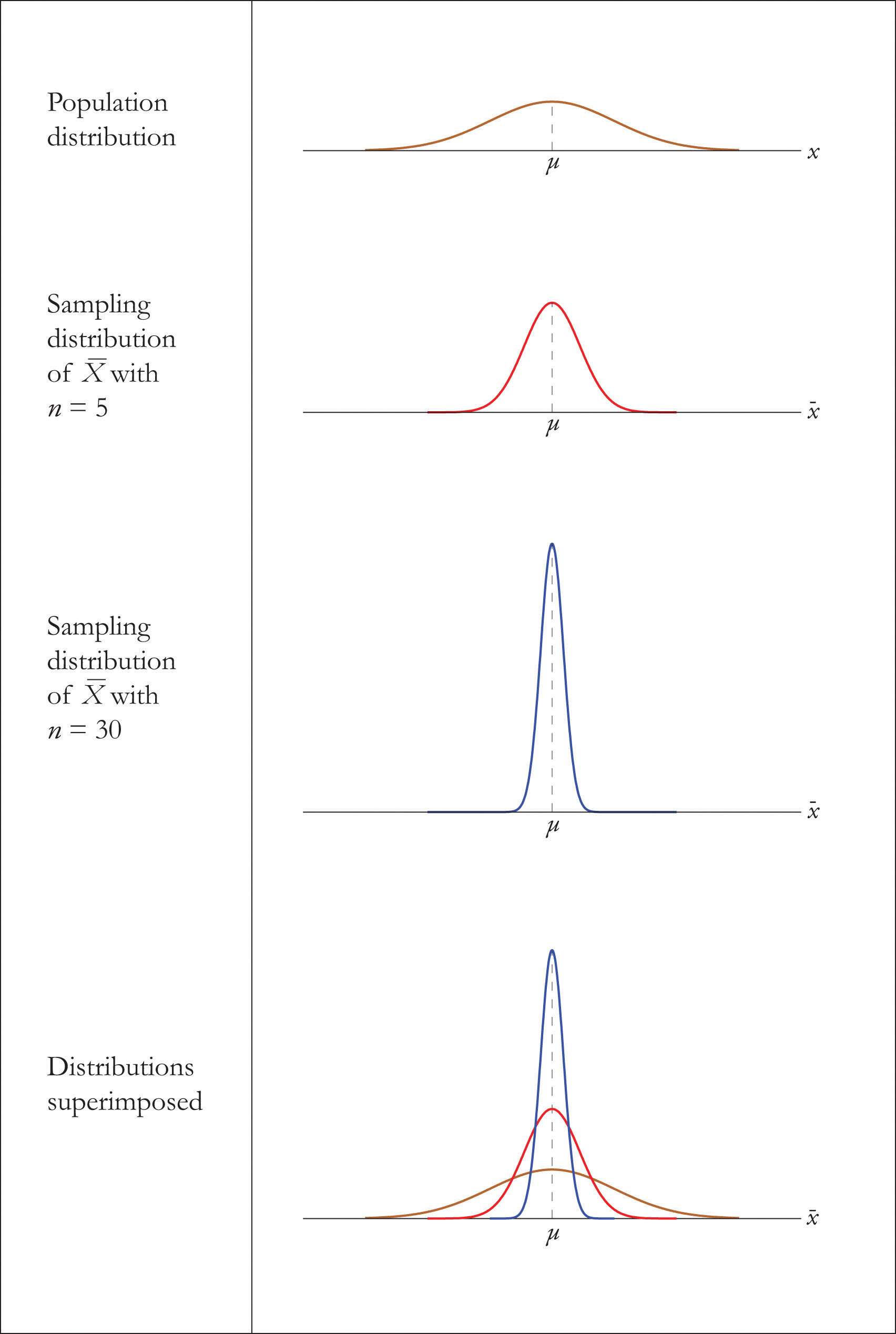
The outcome of increasing the sample size is shown in Figure 6.4 "Distribution of Sample Ways for a Normal Population".

Figure half dozen.4 Distribution of Sample Means for a Normal Population

Case 5

A prototype automotive tire has a blueprint life of 38,500 miles with a standard difference of two,500 miles. Five such tires are manufactured and tested. On the assumption that the actual population mean is 38,500 miles and the bodily population standard difference is 2,500 miles, find the probability that the sample hateful volition be less than 36,000 miles. Assume that the distribution of lifetimes of such tires is normal.

Solution

For simplicity we apply units of thousands of miles. And so the sample mean $\stackrel{-}{\mathit{Ten}}$ has mean ${\mathit{\mu }}_{\stackrel{-}{\mathit{10}}}=\mathit{\mu }=38.5$ and standard deviation ${\mathit{\sigma }}_{\stackrel{-}{\mathit{X}}}=\mathit{\sigma }/\sqrt{n}=\mathrm{two.v}/\sqrt{\mathrm{v}}=1.11803.$ Since the population is usually distributed, so is $\stackrel{-}{\mathit{X}}$ , hence

$$\begin{array}{ll}P(\stackrel{-}{\mathit{X}}<36)\hfill & =P\left(Z<\frac{36-{\mathit{\mu }}_{\stackrel{-}{\mathit{10}}}}{{\mathit{\sigma }}_{\stackrel{-}{\mathit{X}}}}\right)\hfill \\ \hfill & =P\left(Z<\frac{36-38.5}{1.11803}\right)\hfill \\ \hfill & =P\left(Z<\text{−}2.24\right)=0.0125\hfill \end{array}$$

That is, if the tires perform as designed, there is only near a 1.25% gamble that the boilerplate of a sample of this size would exist and so low.

Example 6

An motorcar battery manufacturer claims that its midgrade bombardment has a hateful life of 50 months with a standard deviation of 6 months. Suppose the distribution of battery lives of this particular brand is approximately normal.

1. On the assumption that the manufacturer'southward claims are truthful, find the probability that a randomly selected battery of this blazon volition last less than 48 months.
2. On the same supposition, find the probability that the hateful of a random sample of 36 such batteries volition be less than 48 months.

Solution

1. Since the population is known to have a normal distribution

   $$\begin{array}{ll}P\left(X<48\right)\hfill & =P\left(Z<\frac{48-\mathit{\mu }}{\mathit{\sigma }}\right)=P\left(Z<\frac{48-50}{6}\right)\hfill \\ \hfill & =P\left(Z<\text{−}0.33\right)=0.3707\hfill \end{array}$$

2. The sample mean has mean ${\mathit{\mu }}_{\stackrel{-}{\mathit{10}}}=\mathit{\mu }=50$ and standard deviation ${\mathit{\sigma }}_{\stackrel{-}{\mathit{X}}}=\mathit{\sigma }/\sqrt{\mathrm{northward}}=\mathrm{six}/\sqrt{36}=\mathrm{one}.$ Thus

   $$\begin{array}{ll}P\left(\stackrel{-}{\mathit{10}}<48\right)\hfill & =P\left(Z<\frac{48-{\mathit{\mu }}_{\stackrel{-}{\mathit{Ten}}}}{{\mathit{\sigma }}_{\stackrel{-}{\mathit{X}}}}\right)\hfill \\ \hfill & =P\left(Z<\frac{48-\mathrm{fifty}}{1}\right)\hfill \\ \hfill & =P\left(Z<\text{−}2\right)=0.0228\hfill \end{array}$$

Fundamental Takeaways

• When the sample size is at least 30 the sample mean is commonly distributed.
• When the population is normal the sample mean is normally distributed regardless of the sample size.

Exercises

Basic

1. A population has mean 128 and standard departure 22.

   1. Find the mean and standard deviation of $\stackrel{-}{\mathit{X}}$ for samples of size 36.
   2. Notice the probability that the hateful of a sample of size 36 will be within 10 units of the population mean, that is, between 118 and 138.

2. A population has mean ane,542 and standard deviation 246.

   1. Observe the mean and standard deviation of $\stackrel{-}{\mathit{X}}$ for samples of size 100.
   2. Find the probability that the mean of a sample of size 100 will be within 100 units of the population mean, that is, betwixt 1,442 and one,642.

3. A population has mean 73.5 and standard divergence 2.5.

   1. Find the mean and standard divergence of $\stackrel{-}{\mathit{10}}$ for samples of size 30.
   2. Observe the probability that the mean of a sample of size 30 will exist less than 72.

4. A population has hateful 48.four and standard difference half-dozen.3.

   1. Find the mean and standard deviation of $\stackrel{-}{\mathit{X}}$ for samples of size 64.
   2. Detect the probability that the mean of a sample of size 64 will exist less than 46.7.

5. A normally distributed population has mean 25.half-dozen and standard divergence 3.3.

   1. Find the probability that a unmarried randomly selected element 10 of the population exceeds 30.
   2. Find the mean and standard deviation of $\stackrel{-}{\mathit{X}}$ for samples of size 9.
   3. Discover the probability that the mean of a sample of size 9 fatigued from this population exceeds xxx.

6. A normally distributed population has mean 57.7 and standard deviation 12.1.

   1. Discover the probability that a single randomly selected element X of the population is less than 45.
   2. Find the mean and standard deviation of $\stackrel{-}{\mathit{X}}$ for samples of size xvi.
   3. Find the probability that the hateful of a sample of size 16 drawn from this population is less than 45.

7. A population has mean 557 and standard divergence 35.

   1. Find the mean and standard deviation of $\stackrel{-}{\mathit{X}}$ for samples of size 50.
   2. Find the probability that the mean of a sample of size l will be more than 570.

8. A population has hateful 16 and standard difference i.7.

   1. Find the mean and standard deviation of $\stackrel{-}{\mathit{X}}$ for samples of size lxxx.
   2. Discover the probability that the mean of a sample of size 80 will exist more than 16.iv.

9. A normally distributed population has mean 1,214 and standard deviation 122.

   1. Observe the probability that a single randomly selected element 10 of the population is between 1,100 and 1,300.
   2. Find the mean and standard deviation of $\stackrel{-}{\mathit{X}}$ for samples of size 25.
   3. Find the probability that the mean of a sample of size 25 fatigued from this population is between 1,100 and 1,300.

10. A unremarkably distributed population has mean 57,800 and standard divergence 750.

    1. Detect the probability that a single randomly selected chemical element X of the population is betwixt 57,000 and 58,000.
    2. Find the mean and standard deviation of $\stackrel{-}{\mathit{X}}$ for samples of size 100.
    3. Find the probability that the mean of a sample of size 100 drawn from this population is between 57,000 and 58,000.

11. A population has mean 72 and standard divergence 6.

    1. Find the hateful and standard difference of $\stackrel{-}{\mathit{X}}$ for samples of size 45.
    2. Find the probability that the hateful of a sample of size 45 will differ from the population hateful 72 by at least 2 units, that is, is either less than seventy or more than 74. (Hint: One way to solve the problem is to beginning detect the probability of the complementary event.)

12. A population has mean 12 and standard deviation one.v.

    1. Find the mean and standard deviation of $\stackrel{-}{\mathit{10}}$ for samples of size 90.
    2. Find the probability that the mean of a sample of size 90 will differ from the population mean 12 by at least 0.3 unit, that is, is either less than xi.vii or more 12.iii. (Hint: 1 way to solve the problem is to kickoff find the probability of the complementary event.)

Applications

13. Suppose the mean number of days to germination of a diverseness of seed is 22, with standard deviation 2.iii days. Find the probability that the mean germination fourth dimension of a sample of 160 seeds will exist within 0.five solar day of the population mean.

14. Suppose the mean length of fourth dimension that a caller is placed on hold when telephoning a customer service heart is 23.viii seconds, with standard deviation four.6 seconds. Find the probability that the mean length of time on hold in a sample of i,200 calls will be within 0.5 second of the population mean.

15. Suppose the mean amount of cholesterol in eggs labeled "large" is 186 milligrams, with standard deviation 7 milligrams. Find the probability that the mean corporeality of cholesterol in a sample of 144 eggs will exist within 2 milligrams of the population mean.

16. Suppose that in 1 region of the country the hateful amount of credit card debt per household in households having credit card debt is $xv,250, with standard deviation $7,125. Find the probability that the mean amount of credit carte du jour debt in a sample of 1,600 such households will be within $300 of the population hateful.

17. Suppose speeds of vehicles on a item stretch of roadway are ordinarily distributed with mean 36.6 mph and standard deviation 1.7 mph.

    1. Detect the probability that the speed X of a randomly selected vehicle is between 35 and 40 mph.
    2. Find the probability that the hateful speed $\stackrel{-}{\mathit{X}}$ of 20 randomly selected vehicles is between 35 and xl mph.

18. Many sharks enter a land of tonic immobility when inverted. Suppose that in a detail species of sharks the time a shark remains in a country of tonic immobility when inverted is unremarkably distributed with mean 11.2 minutes and standard departure 1.i minutes.

    1. If a biologist induces a state of tonic immobility in such a shark in order to report it, find the probability that the shark will remain in this state for between 10 and 13 minutes.
    2. When a biologist wishes to estimate the mean time that such sharks stay immobile by inducing tonic immobility in each of a sample of 12 sharks, observe the probability that mean time of immobility in the sample will be between x and 13 minutes.

19. Suppose the mean cost beyond the country of a 30-mean solar day supply of a generic drug is $46.58, with standard deviation $4.84. Find the probability that the hateful of a sample of 100 prices of 30-day supplies of this drug will be between $45 and $50.

20. Suppose the mean length of time between submission of a state tax return requesting a refund and the issuance of the refund is 47 days, with standard deviation 6 days. Notice the probability that in a sample of 50 returns requesting a refund, the hateful such time will be more than 50 days.

21. Scores on a common final examination in a large enrollment, multiple-section freshman course are normally distributed with hateful 72.seven and standard deviation 13.one.

    1. Notice the probability that the score X on a randomly selected exam paper is between seventy and 80.
    2. Find the probability that the hateful score $\stackrel{-}{\mathit{10}}$ of 38 randomly selected exam papers is between 70 and lxxx.

22. Suppose the mean weight of school children's bookbags is 17.4 pounds, with standard departure ii.2 pounds. Notice the probability that the hateful weight of a sample of 30 bookbags volition exceed 17 pounds.

23. Suppose that in a certain region of the state the mean duration of first marriages that end in divorce is 7.eight years, standard deviation 1.2 years. Find the probability that in a sample of 75 divorces, the mean age of the marriages is at well-nigh eight years.

24. Borachio eats at the same fast food restaurant every day. Suppose the time Ten between the moment Borachio enters the eatery and the moment he is served his food is normally distributed with hateful 4.ii minutes and standard difference 1.iii minutes.

    1. Observe the probability that when he enters the eatery today it volition be at least v minutes until he is served.
    2. Notice the probability that average time until he is served in eight randomly selected visits to the restaurant volition be at least 5 minutes.

Additional Exercises

25. A loftier-speed packing machine can exist set to deliver between 11 and 13 ounces of a liquid. For any commitment setting in this range the amount delivered is normally distributed with mean some amount μ and with standard deviation 0.08 ounce. To calibrate the machine it is set to deliver a item amount, many containers are filled, and 25 containers are randomly selected and the amount they contain is measured. Find the probability that the sample hateful volition be inside 0.05 ounce of the actual mean amount being delivered to all containers.

26. A tire manufacturer states that a sure type of tire has a mean lifetime of sixty,000 miles. Suppose lifetimes are commonly distributed with standard deviation $\mathit{\sigma }=\text{3,500}$ miles.

    1. Find the probability that if you purchase 1 such tire, information technology will last only 57,000 or fewer miles. If you had this feel, is it specially strong evidence that the tire is non as good equally claimed?
    2. A consumer group buys five such tires and tests them. Observe the probability that average lifetime of the v tires volition exist 57,000 miles or less. If the mean is so low, is that particularly strong bear witness that the tire is not as good every bit claimed?

Answers

1. 1. ${\mathit{\mu }}_{\stackrel{-}{\mathit{Ten}}}=128$ , ${\mathit{\sigma }}_{\stackrel{-}{\mathit{X}}}=\mathrm{three.67}$
   2. 0.9936
3. 1. ${\mathit{\mu }}_{\stackrel{-}{\mathit{Ten}}}=73.5$ , ${\mathit{\sigma }}_{\stackrel{-}{\mathit{X}}}=0.456$
   2. 0.0005
5. 1. 0.0918
   2. ${\mathit{\mu }}_{\stackrel{-}{\mathit{X}}}=25.6$ , ${\mathit{\sigma }}_{\stackrel{-}{\mathit{X}}}=1.1$
   3. 0.0000
7. 1. ${\mathit{\mu }}_{\stackrel{-}{\mathit{X}}}=557$ , ${\mathit{\sigma }}_{\stackrel{-}{\mathit{Ten}}}=4.9497$
   2. 0.0043
9. 1. 0.5818
   2. ${\mathit{\mu }}_{\stackrel{-}{\mathit{X}}}=1214$ , ${\mathit{\sigma }}_{\stackrel{-}{\mathit{X}}}=\mathrm{24.four}$
   3. 0.9998
11. 1. ${\mathit{\mu }}_{\stackrel{-}{\mathit{X}}}=72$ , ${\mathit{\sigma }}_{\stackrel{-}{\mathit{X}}}=0.8944$
    2. 0.0250

13. 0.9940

15. 0.9994

17. 1. 0.8036
    2. 1.0000

19. 0.9994

21. 1. 0.2955
    2. 0.8977

23. 0.9251

25. 0.9982

How Many Different Samples Of Size 4 Can Be Selected From A Population Of Size 8?,

Source: https://saylordotorg.github.io/text_introductory-statistics/s10-02-the-sampling-distribution-of-t.html

Posted by: pattersonwirciang.blogspot.com

Share this post